Bitemporal Data
A guide to bitemporal data modeling, the advanced technique of tracking data across two distinct timelines (valid time and transaction time) to accurately recreate historical states and track retroactive corrections.
Tracking Two Dimensions of Time
In standard data warehousing, tracking historical changes is typically handled via Slowly Changing Dimensions (SCD Type 2). When a customer’s address changes, a new row is inserted with effective_date and expiration_date columns. This answers the question: “Where did the customer live on January 15th?”
However, standard SCD Type 2 fails when dealing with retroactive corrections. Imagine a customer moved to New York on January 1st. On February 1st, the data entry clerk realizes they made a typo and the customer actually moved to New Jersey on January 1st, and corrects the record.
If an auditor asks, “What did our database think the customer’s address was on January 15th?”, standard SCD Type 2 struggles. The database has been corrected to show New Jersey since Jan 1st. The fact that the database temporarily contained incorrect information has been lost.
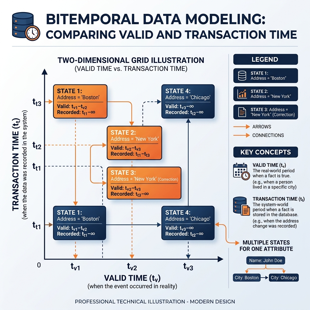
Bitemporal data modeling solves this by tracking data across two entirely independent timelines simultaneously:
1. Valid Time (State Time): The time period when the fact was true in the real world. (e.g., The customer actually lived in New Jersey starting Jan 1st).
2. Transaction Time (Assertion Time): The time period when the database recorded the fact. (e.g., The database recorded the New Jersey address on Feb 1st).
The Bitemporal Schema
A bitemporal table requires four timestamp columns to define the two dimensions of time:
valid_fromvalid_totransaction_fromtransaction_to
When the initial incorrect data entry happens on Jan 1st:
The system inserts a row: Address=New York, valid_from=Jan 1, valid_to=Infinity. transaction_from=Jan 1, transaction_to=Infinity.
When the correction happens on Feb 1st:
The system “retires” the first row by updating its transaction_to to Feb 1st. (This record is now a historical artifact of what the database used to believe).
The system inserts a new row with the correct data: Address=New Jersey, valid_from=Jan 1, valid_to=Infinity. transaction_from=Feb 1, transaction_to=Infinity.
Querying Bitemporal Data
By querying across both timelines, analysts can answer highly complex audit questions:
“As-Of” Queries: “What is the true state of the world as of today?” (Query where today falls between valid_from and valid_to, AND today falls between transaction_from and transaction_to).
“As-Was” Queries: “What did the database think the state of the world was on January 15th?” (Query where Jan 15 falls between valid_from and valid_to, AND Jan 15 falls between transaction_from and transaction_to). This will return the incorrect “New York” record, perfectly recreating the state of the system for compliance auditing.
Bitemporal vs. Apache Iceberg Time Travel
Apache Iceberg provides built-in “Time Travel,” allowing users to query past snapshots of a table. Iceberg Time Travel natively handles the Transaction Time dimension: it allows you to see the database exactly as it existed at a past timestamp.
However, Iceberg Time Travel does not automatically handle Valid Time (when the event actually happened in the real world). To achieve true bitemporal modeling in a lakehouse, data engineers must explicitly model the valid_from/valid_to columns in the table schema, while relying on Iceberg’s snapshot history to handle the transaction_from/transaction_to dimension inherently, drastically simplifying the implementation of this complex modeling pattern.
Learn More
To dive deeper into these architectures and master the modern data ecosystem, check out the comprehensive books by Alex Merced available in our Books section.