Why Operational Schemas Break Analytics

Every operational database is designed with a single priority: transactional write performance. Systems powering e-commerce checkouts, bank transactions, and hospital records use heavily normalized schemas, meaning each piece of information is stored in exactly one place. A customer’s name, address, and email exist in the customers table. Their orders exist in the orders table. Each order’s line items exist in order_items. Products are in a products table, and categories in a separate categories table. This normalization prevents data anomalies when records are updated; change a customer’s email once in the customers table and it is correct everywhere.

The problem emerges the moment an analyst tries to write an analytical query. Answering “How much revenue did we generate from electronics customers in the Northeast region last quarter?” requires joining at least six tables across tens of millions of rows. The SQL query becomes a sprawling tangle of joins, subqueries, and aggregations that is easy to write incorrectly, nearly impossible for a business user to understand, and extremely slow to execute in a database optimized for single-row operations rather than aggregate scans.

Ralph Kimball, working at Xerox’s Palo Alto Research Center and later at his own consulting firm, spent decades studying why business intelligence projects failed. His conclusion was consistent: the schema design imposed on analysts was wrong for analytical work. His solution was dimensional modeling, a deliberately denormalized structure that organizes data the way humans think about business rather than the way databases minimize redundancy.

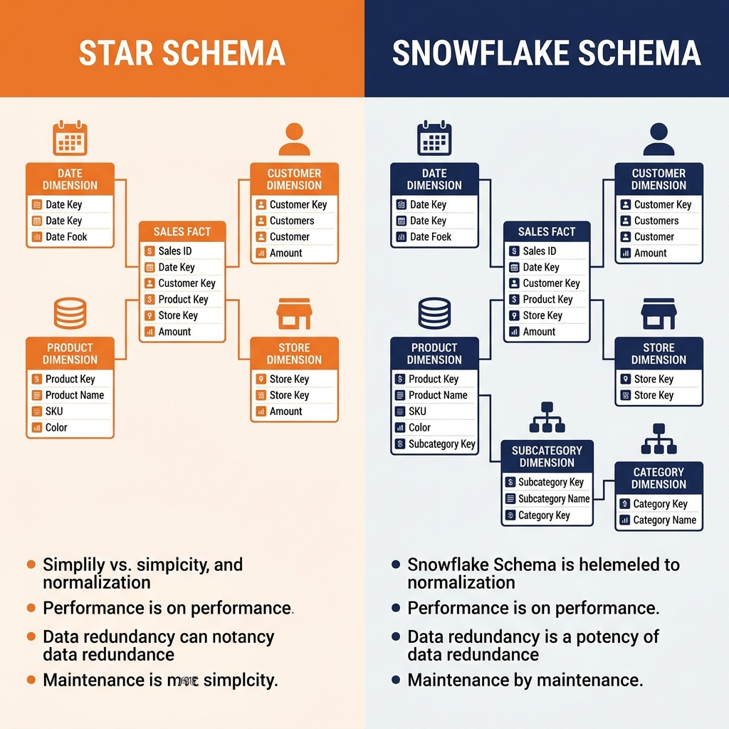
Dimensional modeling has two primary implementations: the Star Schema and the Snowflake Schema. Both organize data around a central Fact table surrounded by Dimension tables, differing only in how much they normalize the Dimension tables themselves.

The Star Schema in Depth

The Star Schema gets its name from its visual representation: a central Fact table radiating outward to Dimension tables through foreign key relationships, forming a star shape. This structure is intentionally denormalized compared to an operational OLTP schema, trading storage efficiency for query simplicity and speed.

Fact Tables: Measuring Business Events

The Fact table is the analytical core of the Star Schema. Every row in a Fact table represents a single measurable business event: a sales transaction, a web page view, a customer service call, a sensor reading, or an insurance claim. Fact tables have two categories of columns.

Degenerate dimensions are keys that link each fact row to the associated Dimension rows. A sales fact row has a date_key pointing to the Date Dimension, a customer_key pointing to the Customer Dimension, a product_key pointing to the Product Dimension, and a store_key pointing to the Store Dimension.

Measures are the numerical values being analyzed. The same sales fact row holds quantity_sold, unit_price, discount_amount, gross_revenue, and cost_of_goods_sold. These are additive facts, meaning they can be meaningfully summed across any combination of dimensions. Analysts can sum gross_revenue by region, by product category, by week, or any combination, because the measure is intrinsically additive.

Fact tables are almost always the largest tables in a dimensional model. A retail chain processing one million transactions per day accumulates 365 million rows per year in the sales fact table, and fact tables spanning decades in high-volume businesses contain hundreds of billions of rows. This scale is exactly why schema optimization matters so much: the Dimension foreign keys are stored as compact integers (4-8 bytes), not duplicated descriptive strings.

Dimension Tables: Providing Context

Dimension tables surround the Fact table and provide the descriptive context for analytical queries. They answer the “who, what, when, where, and how” questions about each business event.

The Date Dimension is the most universally present Dimension in any enterprise star schema. Rather than storing raw timestamp values in the Fact table and deriving date attributes at query time, the Date Dimension pre-computes every possible date attribute for every date in a thirty-year window: day_of_week, week_number, month_name, calendar_quarter, fiscal_quarter, fiscal_year, is_holiday, is_weekend. This pre-computation makes filtering and grouping by time periods trivially fast.

The Customer Dimension stores demographic and behavioral attributes: customer_name, city, state, postal_code, customer_segment, acquisition_channel, registration_date. Because these attributes are stored in the Dimension rather than duplicated in every Fact row, changing a customer’s segment classification requires updating one Dimension row rather than millions of Fact rows.

Querying the Star Schema

The query simplicity advantage of the Star Schema is dramatic. The six-table join nightmare from the normalized operational schema becomes a clean, readable query joining the Fact table to the relevant Dimensions, filtering on Dimension attributes, and summing Fact measures. A SQL query that requires 40 lines against a normalized operational schema often requires only 10 lines against a Star Schema, and it executes dramatically faster because the Dimension joins are optimized lookups from compact integer keys to small lookup tables.

Modern columnar query engines (Dremio, Trino, DuckDB) are specifically tuned to exploit the Star Schema structure. They use Bloom filters and hash join optimizations that treat the small Dimension tables as broadcast hash tables, joining them against the large Fact tables without disk spills.

The Snowflake Schema

The Snowflake Schema is a variant of the Star Schema where Dimension tables are themselves normalized into sub-dimension tables, creating a structure that visually resembles a snowflake. In a Star Schema, the Product Dimension might contain product_name, subcategory_name, and category_name all in a single denormalized table. In a Snowflake Schema, the Product Dimension contains only product_name and a subcategory_key, which references a ProductSubcategory table containing subcategory_name and a category_key, which in turn references a ProductCategory table containing category_name.

The Snowflake Schema reduces storage through normalization, eliminating the repetition of category_name across thousands of Product Dimension rows that belong to the same category. It also makes updating category information cleaner: changing a category name requires updating one row in the ProductCategory table rather than thousands of rows in the Product Dimension.

The trade-off is query complexity. Queries against a Snowflake Schema require additional joins to navigate the sub-dimension hierarchy, adding join overhead to every query. For most enterprise BI environments, the storage savings of the Snowflake Schema are minor compared to the total data volume (Dimension tables are small relative to Fact tables), while the additional join complexity meaningfully degrades query performance and developer experience.

Most dimensional modeling practitioners recommend the Star Schema for its superior query performance and simplicity, reserving the Snowflake Schema for cases where a specific Dimension hierarchy has genuinely large cardinality and the normalization produces a meaningful storage or update management benefit.

Dimensional Modeling in the Apache Iceberg Lakehouse

Dimensional models built on Apache Iceberg tables gain capabilities that traditional data warehouse dimensional models cannot match. Iceberg’s MERGE INTO statement provides the mechanism for applying Slowly Changing Dimension (SCD) Type 2 updates atomically, preserving historical dimension rows while adding new rows reflecting attribute changes. Iceberg Time Travel allows analysts to query the Fact table and Dimension tables as of any historical snapshot, enabling fully accurate as-of-date analytical queries that answer “What did we know about our customers as of January 1st of last year?”

Dremio’s Semantic Layer sits on top of the physical Iceberg-backed dimensional model to provide the final governance layer. Data engineers create Virtual Datasets in Dremio that join Fact tables to their Dimension tables and expose the results under business-friendly column names. Row-level security policies ensure that regional managers can only query Fact rows where the region_key maps to their authorized territory. Data Reflections pre-compute the most common fact-to-dimension join patterns, delivering sub-second BI dashboard performance against petabyte-scale Fact tables backed by Iceberg Parquet files on cloud object storage.

Learn More

To dive deeper into these architectures and master the modern data ecosystem, check out the comprehensive books by Alex Merced available in our Books section.